

2D Seismic Reflection Data Interpretation(Part-II)
Types Of Rocks
Types Of Rocks & Physical Processes Can Be Interpreted By The Crossplots Of Poisson’s Ratio And Vp / Vs Ratio

Lower Goru Scenario
The Lower Goru Position Has Been Determined By The Same Properties, It Lies In The Intermediate Rock Type As The Poisson’s Ratio And Vp / Vs Ratio Values Lies In That Range

P-S Reflectivities
The P-S Reflectivity Contrast With Varying Angle Of Reflectivity Is Strongest For Soft Rocks And Weakest For Hard Rocks. This is Due To Increasing Softness Of Soft Rocks

Differentiated Seismic Section
Seismic Section Was Differentiated Into Soft, Intermediate And Hard Rock Type By Plotting The Results Of Each CDP Against Time

Part-IV
Stratigraphic Description Of Lower Goru Formation By Rock Physics
The Rock Physics Parameters
The Contouring Of Rock Physics Parameters i.e P-Wave Velocity, S-Wave Velocity, Shear Modulus, Bulk Modulus, Poisson’s Ratio And Vp / Vs Ratio has been performed. The Central portion of the figures have closures. These closures suggest the anomalous zone. By combining all the Rock Physics parameters we can assign the lithology to the anomalous zone and may suggest the presence of gas.
Contours Of P-Wave Velocity

Contours Of Poisson’s Ratio
We Can Suggest The Type Of Lithology From The Values Of Poisson’s Ratio, The Closures Of Values Ranging Between 0.23-0.27 Suggest The Presence Of Sand Bodies, Many Gas Wells Are Located Inside These Closed Contours, Indicating The Presence Of Gas Sand Bodies In This Area

Contours Of Shear Modulus

Contours Of Vp / Vs Ratio
Vp / Vs Is Another Lithology Indicator. We Can Detect The Presence Of Gas Sands In The Subsurface

Lithology Map
Lithology Map Has Been Prepared By The Combined Interpretation Of Rock Physics Parameters. The Lithologies Are Identified By The Values Of Poisson's Ratio. These Separate Lithologic Zones Are Given Names On The Basis Of Values Of Vp / Vs

2D Seismic Reflection Data Interpretation(Part-I)
2D Seismic Reflection Data Interpretation
Imaging The Varied Lithology By Using Converted Shear Waves
(Lower Goru As A Case Study)
Imaging The Varied Lithology By Using Converted Shear Waves
(Lower Goru As A Case Study)
Objectives
1) Dividing The Rocks Of The Area By Using Rock Physics
1) Determining The Subsidence By Using Statistical Regression
2) Stratigraphic Description Of The Lower Goru Formation By Using Rock Physics
GEOLOGY OF THE AREA


STRATIGRAPHY (Ahmed et al, 2004)

INTERPRETATION SCHEME
PART – I
Conversion Of Seismic Time Section To Depth Section
PART-II
Division Of Rock Types By Using Rock Physics As A Tool
PART-III
Determining The Subsidence By Using Statistical Regression
PART-IV
Stratigraphic Description Of Lower Goru Formation By Rock Physics
PART-V
The Hydrocarbon Zones And Rock Physics
PART-I
Conversion Of Seismic Time Section To Depth Section
BASEMAP

SEISMIC TIME SECTIONTime Section is the Developed Section of Reflectors Which Shows Subsurface Structure In Time Domain

AVERAGE VELOCITY GRAPH

MEAN VELOCITY GRAPH
Average Velocity Graph Shows The Variation Of Velocity With Time Which Is The Mean Of All CDP’s At The Same Time

DEPTH SECTION
Depth Section Has Been Prepared By The Conversion Of Time Section By Using The Method Of Mean Average. It Shows The Subsurface Structure In Depth Domain

INTERPRETATION
From Time Section And Depth Section We Can See That The Area Has Been Traversed By Normal Faults Forming Horst & Graben Structures. Somewhere step faults can be seen. This means that area has been operated by extensional forces and are more prominent near the boundary between Jacobabad-Khairpur High And Panno-Aqil Graben. Structural Traps May be present in the area provided if they are correlated with the Temperature Gradient.
PART-II
Division Of Rock Types By Using Rock Physics As A Tool
Division Of Rock Types By Using Rock Physics As A Tool
The Poisson’s Ratio
б = 0.5 * (Vp2 – 2 Vs2) / (Vp2 – Vs2)
Where
б = Poisson’s Ratio
Vp = P – Wave Velocity
Vs = S -- Wave Velocity
The Vp / Vs Ratio
Vp / Vs = SQRT (K / µ + 4 / 3)
Where
K = Bulk Modulus
µ = Shear Modulus
The Bulk Modulus
K = ρ * (Vp2 - 4 / 3 Vs2)
Where
Vp = P – Wave Velocity
Vs = S – Wave Velocity
The Shear Modulus
µ = ρ * Vs2
Where
ρ = Density
Vs = Shear Wave Velocity
Calculations For CDP 1256

Sequence Stratigraphy(Part-III)
2- SURFACES
i) Sequence boundaries
A sequence boundary is a surface that separates older sequences from younger ones. Commonly it is an unconformity (indicating subaerial exposure), but in limited cases a correlative conformable surface. In other words, the sequences are enveloped by the sequence boundaries (SB). These boundaries are the product of a fall in sea level that erodes the subaerially exposed sediment surface of the earlier sequence or sequences.
Two distinct types of sequence boundary are recognized. Type-1 sequence boundaries equate to those formed during a forced regression whereas Type-2 sequence boundaries are those formed during a normal regression. Type 1 and Type 2 unconformities can bound the same sequence at different localities and are the products of different rates of sedimentation and accommodation space for the same time interval.
ii) Transgressive Surface (TS)
This is a marine-flooding surface that forms the first significant flooding surface in a sequence. In most siliciclastic and some carbonate successions, it marks the onset of the period when the rate of creation of accommodation space is greater than the rate of sediment supply. It forms the base of the retrogradational parasequence stacking patterns of the Transgressive Systems Tract (TST). In areas of high sediment supply, e.g. on rimmed carbonate platforms, the rate of sediment supply may keep pace with the rate of relative sea-level rise and thus the TS will mark a change from a progradational to an aggradational parasequence stacking patterns.
A transgressive surface is often characterized by the presence of a surface marked by consolidated muds of firmgrounds or hardgrounds that are cemented by carbonates. Both surfaces are often penetrated by either burrowing or boring organisms.
If the rate of sediment supply is low over the transgressive surface this may merge landward with the maximum flooding surface. When TS extends over LST valley fill, the response on the resistivity log curve may show a small local increase in resistivity followed by a low value. This increase in resistivity is in response to the carbonate cementation of the hardground, while the low is associated with deposition of transgressive shales.
iii) Maximum Flooding Surface (mfs)
A surface of deposition at the time the shoreline is at its maximum landward position (i.e. the time of maximum transgression. It separates the Transgressive and Highstand Systems Tract. Seismically, it is often expressed as a downlap surface. An mfs is often characterized by the presence of radioactive and often organic rich shales, glauconite, and hardgrounds. An mfs can often be the only portion of a sedimentary cycle, which is rich in fauna.
iv) Marine Flooding Surface
It is a surface separating younger from older strata, across which there is evidence of an abrupt increase in water depth. It may also display evidence of minor submarine erosion. It forms in response to an increase in water depth.
v) Regressive Surface of Erosion
It is a subaqueous surface of marine erosion formed during a relative sea-level fall. As sea level falls, wave base and the upper shoreface zone of current transport drops, too, and planes off the seafloor sediments that formerly lay below wave base and the upper shoreface currents. Such a fall usually is followed by the superposition of coarser-grained upper shoreface deposits sharply overlying finer-grained lower shoreface or shelf deposits associated with the following transgression.
Condensed section
A thin marine stratigraphic interval characterized by very slow depositional rates (<1-10 mm/yr). It consists of fine-grained sedimentary rocks such as hemipelagic and pelagic sediments. These are deposited on the middle to outer shelf, slope, and basin floor during a period of maximum relative sea-level rise and maximum transgression of the shoreline. It first begins to form in more distal slope and basinal environments, and as the shoreline backsteps landward, gradually expands in its coverage to include not only the basin but all of the slope and part of the shelf as well.
Commonly the upper layer of the Transgressive Systems Tract is a condensed section which is associated with the mfs where it is overlain by the downlapping Highstand Systems Tract. Sometimes the transgressive surface marking the base of the Trangressive Systems Tract is immediately overlain by a condensed section that is in turn capped by the mfs.
vi) Ravinement Erosional Surface
It is a time transgressive or diachronous subaqueous erosional surface resulting from nearshore marine and shoreline erosion associated with a sea-level rise. This erosional surface parallels the migration of the shoreface "razor" across previously deposited coastal deposits. Burrows in this surface are often filled by sediments deposited during a sea-level rise.
Ravinement surfaces are commonly ascribed to the transgressive movement of the landward margin of the Transgressive Systems Tract. However, these erosional surfaces tend to occur
wherever the landward edge of the sea rises over an underlying sedimentary surface. Thus if the Late Lowstand Systems Tract has a subaerial landward margin it will have an updip ravinement surface associated with it.
wherever the landward edge of the sea rises over an underlying sedimentary surface. Thus if the Late Lowstand Systems Tract has a subaerial landward margin it will have an updip ravinement surface associated with it.
In outcrops and wells ravinement surfaces are commonly equated with the transgressive surface. However, as the attached movie shows, these erosional surfaces are time transgressive and tend to occur wherever the landward edge of the sea rises over an underlying sedimentary surface. They only match the transgressive surface when it tops the shelf margin.
vii) Clinoform, Undaform and Fondoform Surfaces
(1) Undaform stands for any surface underlying an unda environment.
(2) Clinoform stands for any surface underlying a clino environment.
(3) Fondoform stands for any surface underlying a fondo environment.
So clinoform surface can be used for the sloping depositional surface that is commonly associated with strata prograding into deep water.
So clinoform surface can be used for the sloping depositional surface that is commonly associated with strata prograding into deep water.
In 1951, it was the proposed that the depositional settings of sediment accumulation on the shelf, slope, and bottom be called as:
(1) Unda for shallow water overlying the shelf,
(2) Clino for the deeper water overlying the slope, and
(3) Fondo for the deepest water covering the bottom of the basin.
Basin-floor Fan
It is a portion of the lowstand Systems Tract characterized by deposition of submarine fans on the lower slope or basin floor. Fan formation is associated with the erosion of canyons into the slope and the incision of fluvial valleys into the shelf. Siliciclastic sediment bypasses the shelf and slope through the valleys and canyons to feed the basin-floor fan. The basin-floor fan may be deposited at the mouth of a canyon or widely separated from it, or a canyon may not be evident.
Hiatus
A cessation in deposition of sediments during which no strata form or an erosional surface forms on the underlying strata; a gap in the rock record. This period might be marked by development of lithified sediment (hardground) or burrowed surface characteristic of periods when sea level was relatively low. A disconformity can result from a hiatus.
Hardground
A horizon cemented by precipitation of calcite just below the sea floor. Local concretions form first in a hardground and can be surrounded by burrows of organisms until the cement is well developed.
Stacking Patterns
Strike
A direction of line formed by the intersection of a plane, such as a dipping bed, with a horizontal surface
Azimuth
The angle between the vertical projection of a line of interest onto a horizontal surface and true north or magnetic north measured in a horizontal plane, typically measured clockwise from north.
Apparent Dip
The angle that a plane makes with the horizontal measured in any randomly oriented section rather than perpendicular to strike.
Two-dimensional (2-D) survey
Seismic data or a group of seismic lines acquired individually such that there are significant gaps (commonly 1 km or more) between adjacent lines. A 2 D survey typically contains numerous lines acquired orthogonally to the strike of geological structures (such as faults and folds) with a minimum of lines acquired parallel to geological structures to allow line-to-line tying of the seismic data and interpretation and mapping of structures.

Pinch out 1
A type of stratigraphic trap. The termination by thinning or tapering out ("pinching out") of a reservoir against a nonporous sealing rock creates a favorable geometry to trap hydrocarbons, particularly if the adjacent sealing rock is a source rock such as shale.
Pinch out 2
A reduction in bed thickness resulting from onlapping stratigraphic sequences
Seismic Stratigraphy
•Seismic stratigraphy is based on the principle that seismic reflectors follow stratal patterns and approximate isochrons (time lines)
•Reflection terminations provide the data used to identify sequence-stratigraphic surfaces, systems tracts, and their internal stacking patterns
•Technological developments have been prolific:
•Vertical resolution improved to a few tens of meters
•Widespread use of 3D seismic
•Seismic data should preferably always be interpreted in conjunction with well log or core data
•A better understanding of stratigraphic sequences can be obtained by the construction of chronostratigraphic charts (‘Wheeler diagrams’); these can subsequently be used to infer coastal-onlap curves
•Variations in sediment supply can produce stratal patterns that are very similar to those formed by RSL change (except for forced regression); in addition, variations in sediment supply can cause stratigraphic surfaces at different locations to be out of phase
•In principle, sequence-stratigraphic concepts could be applied with some modifications to sedimentary successions that are entirely controlled by climate change and/or tectonics (outside the realm of RSL control).
•The global sea-level curve for the Mesozoic and Cenozoic (inferred from coastal-onlap curves) contains first, second, and third-order eustatic cycles that are supposed to be globally synchronous, but it is a highly questionable generalization
•Conceptual problems: spatially variable RSL change due to differential isostatic and tectonic movements undermines the notion of a globally uniform control
•Dating problems: correlation is primarily based on biostratigraphy that typically has a resolving power comparable to the period of third-order cycles
Recommended procedures for performing seismic sequence analysis include:
1. Identifying the unconformities in the area of interest. Unconformities are recognized as surfaces onto which reflectors converge.
2. Mark these terminations with arrows.
3. Draw the unconformity surface between the onlapping and downlapping reflections above; and the truncating and toplapping reflections below.
4. Extend the unconformity surface over the complete section. If the boundary becomes conformable, trace its position across the section by visually correlating the reflections.
5. Continue identifying the unconformities on all the remaining seismic sections for the basin.
6. Make sure the interpretation ties correctly among all the lines.
7. Identify the type of unconformity:
a. Sequence boundary: this is characterized by regional onlap above and truncation below.
b. Downlap surface: this is characterized by regional downlap.
Recommended color codes:
Red: Reflection patterns and reflection terminations.
Green: Downlap surfaces
Blue: Transgressive surfaces
Other colors: Sequence boundaries
If using only black and white:
Thin solid lines ( ) : Reflection patterns
Dashed lines (---------): Downlap surfaces
Dotted lines ( ………. ): Transgressive surfaces
Sequence stratigraphic application to outcrops
Although sequence stratigraphy was originally designed for seismic sections, sequence principles can be readily applied to outcrop, core, and well logs. The first step in this approach is to interpret individual beds in terms of depositional events, including an evaluation of the shear stress in the environment, the type of flow (currents, waves, tides, and combined flow), bioturbation and trace fossils, etc. This information is critical for the next step, to recognize bedsets, that is groups of beds that record similar depositional processes, and to interpret those bedsets as facies, the records of particular depositional environments. These steps are critical because errors at this point may cause errors in interpretations of relative depth, which in turn affects the recognition of parasequences and stacking patterns. Solid facies work is essential for a solid sequence analysis.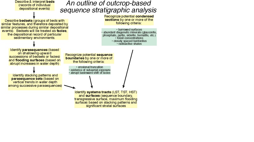
From successions of facies in an outcrop, shallowing-upward successions can be recognized as well as flooding surfaces such that parasequences can be delimited. Vertical trends in the range of water depths present in successive parasequences can be used to identify stacking patterns and to recognize surfaces that mark the turnarounds from one parasequence set to the next. Potential sequence boundaries should be identified at this step based on one or more of the following criteria: clearly defined erosional truncation, direct evidence of subaerial exposure, or abrupt basinward shifts of facies. Likewise, potential condensed sections should be recognized on the basis of unusual burrowed surfaces, abundant diagenetic materials, fossil concentrations, closely spaced bentonite beds, or radioactive shales. Condensed sections may, but do not necessarily, lie along the maximum flooding surface.
From the recognition of parasequence sets and potential sequence boundaries and condensed sections, systems tracts and major stratal surfaces (sequence boundary, transgressive surface, and maximum flooding surface) can be recognized. It is important to stress that not all of these surfaces or systems tracts may be present within any given sequence in an outcrop. The absence of one or more surfaces or systems tracts may provide important clues as to the relative position of the outcrop within the basin. For example, lowstand systems tracts are commonly absent in updip areas where the transgressive surface and sequence boundary are merged as one surface. In such areas, significant portions of the highstand systems tract may have eroded away and the sequence boundary is marked by the beginning of retrogradational stacking. In downdip areas, the transgressive and highstand systems tracts may be thin and relatively mud-rich, whereas the lowstand systems tract may be characterized by the abrupt appearance of thick sandy facies. Many more variations are possible and many basins are characterized by a typical pattern of sequence architecture.

Sequence Stratigraphy(Part-II)
b) For a Muddy Siliciclastic
A parasequence developed on a muddy siliciclastic shoreline would have a different suite of facies, but they would also be arrayed vertically in a shallowing upward order and facies relationships would obey Walther's Law. A typical muddy shoreline parasequence would start with cross-bedded subtidal sands, continue with interbedded bioturbated mudstones and rippled sands of the intertidal, and pass upwards into entirely bioturbated and possibly coaly mudstones of the supratidal.

Parasequence with respect to Flooding Surface
The flooding surfaces that define the top and base of a parasequence display abrupt contacts of relatively deeper-water facies lying directly on top of relatively shallow-water facies. Rocks lying above and below a flooding surface commonly represent non-adjacent facies, such as offshore shales directly overlying foreshore sands or basinal shales directly overlying mid-fan turbidites. Thus, Walther's Law cannot be applied across flooding surfaces. Given that many parasequences are meters to tens of meters thick; this radically reduces the scale at which Walther's Law can be applied. Cases where Walther's Law has been applied to sections hundreds to thousands of meters thick are nearly always incorrect.
Flooding Surface Interpretations
Flooding surfaces may exhibit ;
Ø Small scale erosion, usually of a meter or less.
Ø Flooding surfaces may be mantled by a transgressive lag composed of shells, shale intraclasts, calcareous nodules, or siliciclastic gravel; such lags are usually thin, less than a meter thick.
Ø Flooding surfaces may display evidence of firmgrounds, such as Glossifungites ichnofacies, or hardgrounds that may be bored, encrusted, and possibly mineralized.
Lateral and Vertical Relationships within a Parasequence
One of the most powerful aspects to recognizing parasequences is understanding and applying the predictable vertical and lateral facies relationships within parasequences. Facies reflect increasingly shallower environments upwards within a parasequence. Although a complete vertical succession of facies can be compiled from a suite of parasequences, most parasequences will display only a portion of the entire shallowing-upward succession of facies.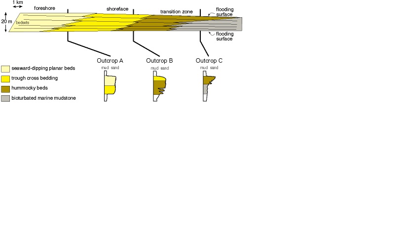
Shallow and Deeper Water Facies
Because shallow water facies within a parasequence will pinch out laterally in a downdip direction and deeper water facies within a parasequence will pinch out in an updip direction, the facies composition of a single parasequence changes predictably updip and downdip. Thus, a single parasequence will not be composed of the same facies everywhere, but will be composed of deeper water facies downdip and shallower water facies updip, as would be expected. Because parasequence boundaries represent a primary depositional surface, that is, topography at the time of deposition, flooding surfaces will tend to be relatively flat but dip slightly seaward at angles typical of continental shelves. Finally, parasequence boundaries may become obscure in coastal plain settings and in deep marine settings because of a lack of facies contrast necessary to make flooding surfaces visible.
Parasequence Sets and Stacking Patterns
In most cases, there will not be simply one parasequence by itself, but there will be a series of parasequences. Sets of successive parasequences may display consistent trends in thickness and facies composition and these sets may be progradational, aggradational, or retrogradational.
a- Progradational Stacking
In a progradational set of parasequences, each parasequence builds out or advances somewhat farther seaward than the parasequence before. Because of this, each parasequence contains a somewhat shallower set of facies than the parasequence before. This produces an overall shallowing-upward trend within the entire parasequence set and the set is referred to as a progradational parasequence set or is said to display progradational stacking. The overall rate of deposition is greater than the rate of accommodation in progradational stacking pattern.
Recognition in a Single Outcrop
In a single outcrop, a progradational parasequence set can be recognized by the progressive appearance of shallower-water facies upward in the parasequence set as well as the progressive loss of deeper-water facies upward in the parasequence set. For example, in a set of progradationally stacked parasequences, perhaps all of the parasequences contain shoreface and foreshore facies, but only the uppermost parasequences may contain the coastal plain coal, and only the lowermost parasequences may contain offshore and transition zone facies.
Recognition in a Cross Section
In a cross-section, a progradational parasequence set can be recognized by the seaward movement of a particular facies contact at an equivalent position in a parasequence. For example, the contact between the shoreline sands and the coastal plain facies at the top of each parasequence will appear to move farther basinward in each successive parasequence. Likewise, the same contact at the base of each parasequence will appear to move farther basinward in each successive parasequence.
b- Aggradational Stacking
In an aggradational set of parsequences, successively younger parasequences are deposited above one another with no significant lateral sifts. The rate of accommodation approximates the rate of deposition. Thus, each parasequence contains essentially the same suite of facies as the parasequences above and below. This lack of overall facies change results in no net vertical trend in water depth. Such a set is called an aggradational parasequence set or is said to display aggradational stacking.
Recognition in a Single Outcrop
In a single outcrop, an aggradational parasequence set can be recognized by the similarity of facies composition in each successive parasequence. No new deeper or shallower water facies will tend to appear near the top or base of the parasequence set.

Recognition in a Cross Section
In a cross-section, an aggradational parasequence set can be recognized by the relative stability of any particular facies contact at an equivalent position in a parasequence. For example, the contact between the shoreline sands and the coastal plain facies at the top of each parasequence will appear to stay at essentially the same position in each successive parasequence. Facies contacts rarely remain at exactly the same position, so aggradational parasequence sets are commonly characterized by relatively minor facies shifts that display no clear long-term trend.
c- Retrogradational Stacking
In a retrogradational set of parasequences, each parasequence progrades less than the preceding parasequence. The result is that each parasequence contains a deeper set of facies than the parasequence below. This net facies shift produces an overall deepening upward trend within the entire parasequence set and the set is referred to as retrogradational parasequence set or is said to display retrogradational stacking. Retrogradational stacking is also commonly called backstepping.
Recognition in a Single Outcrop
In a single outcrop, a retrogradational parasequence set can be recognized by the progressive appearance of deeper water facies upwards within the parasequence set as well as the progressive loss of shallower water facies upwards in the parasequence set. For example, in a set of retrogradationally stacked parasequences, offshore facies might be present in only the uppermost parsequences, and coastal plain coals might be present in only the lowermost parasequence.
Recognition in a Cross Section
In a cross-section, a retrogradational parasequence set can be recognized by the landward movement of a particular facies contact at an equivalent position in a parasequence. For example, the contact between the shoreline sands and the coastal plain facies at the top of each parasequence will appear to move farther landward in each successive parasequence.
DEPOSITIONAL SEQUENCES
“A relatively conformable succession of genetically related strata bounded by unconformities or their correlative conformities”.
Explanation
What the definition does emphasize is that every sequence is bounded above and below by unconformities, or by correlative conformities (surfaces that correlate updip to an unconformity). Every depositional sequence is the record of one cycle of relative sea level. Because of this, depositional sequences have a predictable internal structure consisting of major stratal surfaces and systems tracts, which are suites of coexisting depositional systems, such as coastal plains, continental shelves, and submarine fans.
Compositional Setting
In vertical succession, all depositional sequences are composed of the following elements in this order: sequence boundary, lowstand systems tract, transgressive surface, transgressive systems tract, maximum flooding surface, highstand systems tract, and the following sequence boundary. So, it can be divided into two classes as follows,
1- System Tracts
a- Lowstand Systems Tract (LST)
b- Falling Stage Systems Tract (FSST)
c- Transgressive Systems Tract (TST)
d- Highstand Systems Tract (HST)
2- Surfaces
a- Sequence Boundaries
b- Transgressive Surface
c- Maximum Flooding Surface
1- SYSTEMS TRACT
Genetically associated stratigraphic units that were deposited during specific phases of the relative sea-level cycle form a systems tract. It is a linkage of contemporaneous depositional systems. Each system is defined by stratal geometries at bounding surfaces, position within the sequence, and internal parasequence stacking patterns. Different systems tracts represent different phases of eustatic changes.
a. Lowstand Systems Tract (LST)
The Lowstand Systems Tract is bounded by the Falling Stage Systems Tract (FSST) at the base, and the Transgressive Systems Tract (TST) at the top. It means that this systems tract lies directly on the upper surface of the Falling Stage Systems Tract (FSST) and is capped by the transgressive surface formed when the sediments onlap onto the shelf margin. It is overlain by the transgressive surface (TS) of the overlying TST. These Lowstand Systems Tract sediments form a lowstand wedge and often fill incised valleys that cut down into the Highstand Systems Tract. Because sediments are transported from land to sea, discrete depositional packages, called parasequences, are developed. Beach parasequences typically coarsen upward and in the progradational direction change facies from coastal plain (coal and clay) through marginal marine (sandstone) to offshore.
Traditionally the sediments of this systems tract include the deposits that accumulated after the onset of relative sea-level fall. In contrast to the new Lowstand Systems Tract, the traditional Lowstand Systems Tract lies directly on the sequence boundary over the Highstand Systems Tract. The Lowstand Systems Tract can be divided into Early and Late Phases.
Early Phase Lowstand Systems Tract is associated with:
a. Falling stage of relative sea level induced by eustasy falling rapidly and/or tectonic uplift outpacing the rate of change in sea level position
b. Fluvial incision up dip with formation of an unconformity or sequence boundary and the focus of sediment input at the shoreline
c. Forced regressions induced by the lack of accommodation producing stacking patterns of downward stepping prograding clinoforms over the condensed section formed during the previous transgressive and highstand systems tracts
d. Basin floor fans formed from sediment transported from the shelf margin when this fails under the weight of the rapid sediment accumulation associated with the forced regression
e. Onlap of sediments onto the prograding clinoforms below the shelf break
The lower bounding surfaces of the Early Phase Lowstand System Tract are the updip unconformity and the top of the downdip condensed section. These surfaces form by different mechanisms and have different time significance
The top of the downdip condensed section immediately underlies the downlapping prograding clinoforms of the forced regression
The top of the Early Phase Lowstand System Tract in theory is marked by an initial onlap onto the often eroded surface of the prograding clinoforms of the forced regression
Late Phase Lowstand Systems Tract is associated with:
a. A slow relative sea level rise is induced when eustasy begins to rise slowly and/or tectonic uplift slows
b. Sediment is now outpaced by an increase in accommodation and in response the sediment begins to onlap onto the basin margin
c. River profiles stabilize
d. Valleys backfill
e. Prograding lowstand clinoforms form and are capped by topset layers that onlap, aggrade, become thicker upward and landward
Figure 3. Lowstand systems tract
The old Lowstand Systems Tract is divided into the Falling Stage Systems Tract (FSST) with its basin-floor fans, and slope fans while, the Lowstand Systems Tract sediments form lowstand wedges, often filling incised valleys that cut down into the Highstand Systems Tract. Thus a terminology has been used, which suggests that the sediments of this systems tract can be equated with a relative fall in sea level forming the Falling Stage Systems Tract, and we now refer to the Late Lowstand Systems Tract as the Lowstand Systems Tract because this systems tract is equated with only a small rise in sea level and is an essentially lowstand set of deposits.
b. Falling Stage Systems Tract (FSST)
It includes all the regressional deposits that accumulated after the onset of a relative sea-level fall and before the start of the next relative sea-level rise. The Falling Stage Systems Tract is the product of a forced regression. The FSST lies directly on the type-1 sequence boundary and is capped by the overlying Lowstand Systems Tract sediments. This systems tract has also been termed the Early Lowstand Systems Tract (ELST). On seismic data, the upper boundary is the first definable horizon that onlaps the FSST, but when well logs and outcrops are used this boundary is instead recognized as the first marine-flooding surface that overlies the FSST. Coincidently it is often marked by a time transgressive ravinement surface overlain by a sediment lag.
c. Transgressive Systems Tract (TST)
A transgressive systems comprises the deposits that accumulated from the onset of coastal transgression until the time of maximum transgression of the coast, just prior to the renewed regression of the HST. The TST lies directly on the transgressive surface (TS) formed when the sediments onlap the underlying LST and is overlain by the maximum flooding surface (mfs) formed when marine sediments reach their most landward position. Stacking patterns exhibit backstepping onlapping retrogradational clinoforms that thicken landward. In cases where there is high sediment supply the parasequences may be aggradational.
d- Highstand Systems Tract (HST)
These are the progradational deposits that form when sediment accumulation rates exceed the rate of increase in accommodation space. The HST lies directly on the maximum flooding surface (mfs) formed when marine sediments reached their most landward position. This systems tract is capped by a sequence boundary. The base of HST is formed by the maximum flooding surface (mfs) over which the Highstand Systems Tract sediments prograde and aggrade. The top of this systems tract is formed by the eroded unconformity surface that develops when a sea level fall initiates erosion of the now subaerial Highstand system sediment surface and the start of the Falling Stage Systems Tract.
A highstand systems tract is associated with:
1. Slow rise of relative sea level followed by a slow fall; essentially a still stand of base level when the slower rate eustatic change balances that of tectonic motion
2. Sediment outpacing loss of accommodation
3. River Profiles stabilize
4. River valleys are dispersed laterally in a position landward of the shelf margin.

Figure Highstand systems tract
This systems tract is commonly widespread on the shelf and may be characterized by one or more aggradation to progradational parasequence sets with prograding clinoform geometry. They onlap the sequence boundary in a landward direction and downlap the top of the Transgressive and/or Lowstand Systems Tracts in a basinward direction.

TYPE 1 and TYPE 2 Sequences
Not all relative falls in sea level occur at rates fast enough to expose the continental shelf. For example, during a eustatic fall, a rapidly subsiding margin may still experience a relative rise in sea level, provided the rate of eustatic fall is less than the rate of subsidence. Early seismic studies recognized two types of sequences reflecting the case of sea-level fall below the shelf-slope break (type 1) and the case where sea level does not fall below this break (type 2). Although there has been much subsequent confusion about the application of these two types to outcrop studies, their definitions have been modified such that a type 1 sequence now refers to one in which there is a relative fall in sea level below the position of the present shoreline and a type 2 sequence refers to a sequence in which the relative fall in sea level does not force a shift in the position of the shoreline.
Figure adapted from Van Wagoner et al. (1990)
Type 2 sequences (shown below) are similar to type 1 sequences (shown above) in nearly all regards except for the extent of the sequence-bounding unconformity and its expression in the marine realm. In addition, the two sequences differ in the name of the systems tract lying above the sequence boundary but below the transgressive surface.

Figure adapted from Van Wagoner et al. (1990)
In a type 2 sequence, the extent of the sequence-bounding unconformity can reach seaward only to the position of the previous shoreline, but no further. In other words, none of the marine areas of the previous highstand are subaerially exposed during a type 2 sequence boundary. Updip of these areas, the sequence bounding unconformity is expressed as for a type 1 sequence, but no incised valley forms as sea level does not fall far enough for incision. In the marine realm, no basinward shift of facies occurs as in a type 1 sequence, and the type 2 sequence boundary is characterized only by a slight change in stacking patterns from increasingly progradational in the underlying highstand to decreasingly progradational (possibly aggradational) above the sequence boundary. Detecting this subtle transition in marine sections may be difficult to impossible and many type 2 sequence boundaries probably go undetected.
The shelf margin systems tract in a type 2 sequence is equivalent in stratigraphic position to the lowstand systems tract of a type 1 sequence. As stated above, the shelf margin systems tract is characterized by aggradational stacking. Like the lowstand systems tract, the shelf margin systems tract is capped by the transgressive surface.
In general, far more type 1 sequences have been reported than type 2 sequences, possibly in part reflecting their comparative difficulty or ease of detection. Some workers have gone so far as to question the existence of any type 2 sequences.
Subscribe to:
Posts (Atom)